Photometry

The following examples are adapted from Photometry.jl to show the same examples combined with AstroImages.jl. To learn how to measure background levels, perform aperture photometry, etc., see the Photometry.jl documentation.

Background Estimation

From Photometry.jl:

Estimating backgrounds is an important step in performing photometry. Ideally, we could perfectly describe the background with a scalar value or with some distribution. Unfortunately, it's impossible for us to precisely separate the background and foreground signals. Here, we use mixture of robust statistical estimators and meshing to let us get the spatially varying background from an astronomical photo.

Let's show an example [...]. Now let's try and estimate the background using estimate_background. First, we'll sigma-clip to try and remove the signals from the stars. Then, the background is broken down into boxes, in this case of size (50, 50). Within each box, the given statistical estimators get the background value and RMS. By default, we use SourceExtractorBackground and StdRMS. This creates a low-resolution image, which we then need to resize. We can accomplish this using an interpolator, by default a cubic-spline interpolator via ZoomInterpolator. The end result is a smooth estimate of the spatially varying background and background RMS.

using Photometry
using AstroImages
using Plots # optional, for implot functionality
using Downloads: download

# Download our image, courtesy of astropy
image = load(download("https://rawcdn.githack.com/astropy/photutils-datasets/8c97b4fa3a6c9e6ea072faeed2d49a20585658ba/data/M6707HH.fits"))

# sigma-clip
clipped = sigma_clip(image, 1; fill = NaN)

# get background and background rms with box-size (50, 50)
bkg, bkg_rms = estimate_background(clipped, 50)

We can take a look at each of our processed images with imview:

imview([image; clipped])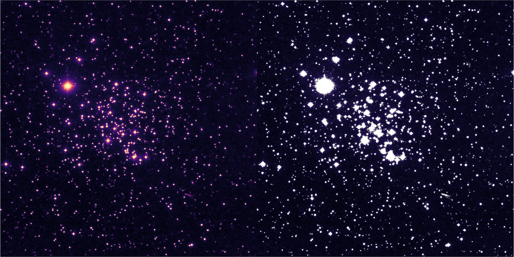

imview([bkg; bkg_rms])

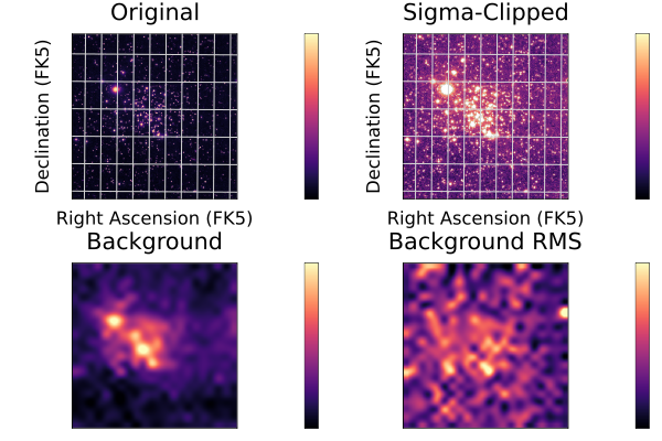
Or all together with Plots.jl:

using Plots

AstroImages.set_clims!(Percent(99.5))
AstroImages.set_cmap!(:magma)
AstroImages.set_stretch!(identity)

plot(
    implot(image; title = "Original"),
    implot(clipped; title = "Sigma-Clipped"),
    implot(bkg; title = "Background"),
    implot(bkg_rms; title = "Background RMS");
    layout = (2, 2),
    ticks = false,
)

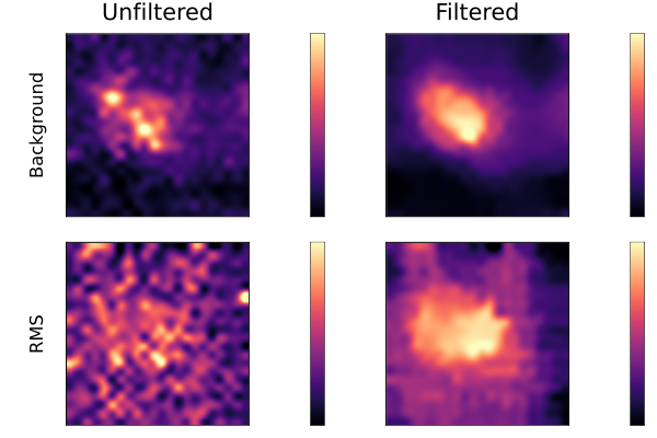
We could apply a median filter, too, by specifying filter_size:

# get background and background rms with box-size (50, 50) and filter_size (5, 5)
bkg_f, bkg_rms_f = estimate_background(clipped, 50; filter_size = 5)

# plot
plot(
    implot(bkg; title = "Unfiltered", ylabel = "Background"),
    implot(bkg_f; title = "Filtered"),
    implot(bkg_rms; ylabel = "RMS"),
    implot(bkg_rms_f);
    layout = (2, 2),
    ticks = false,
)

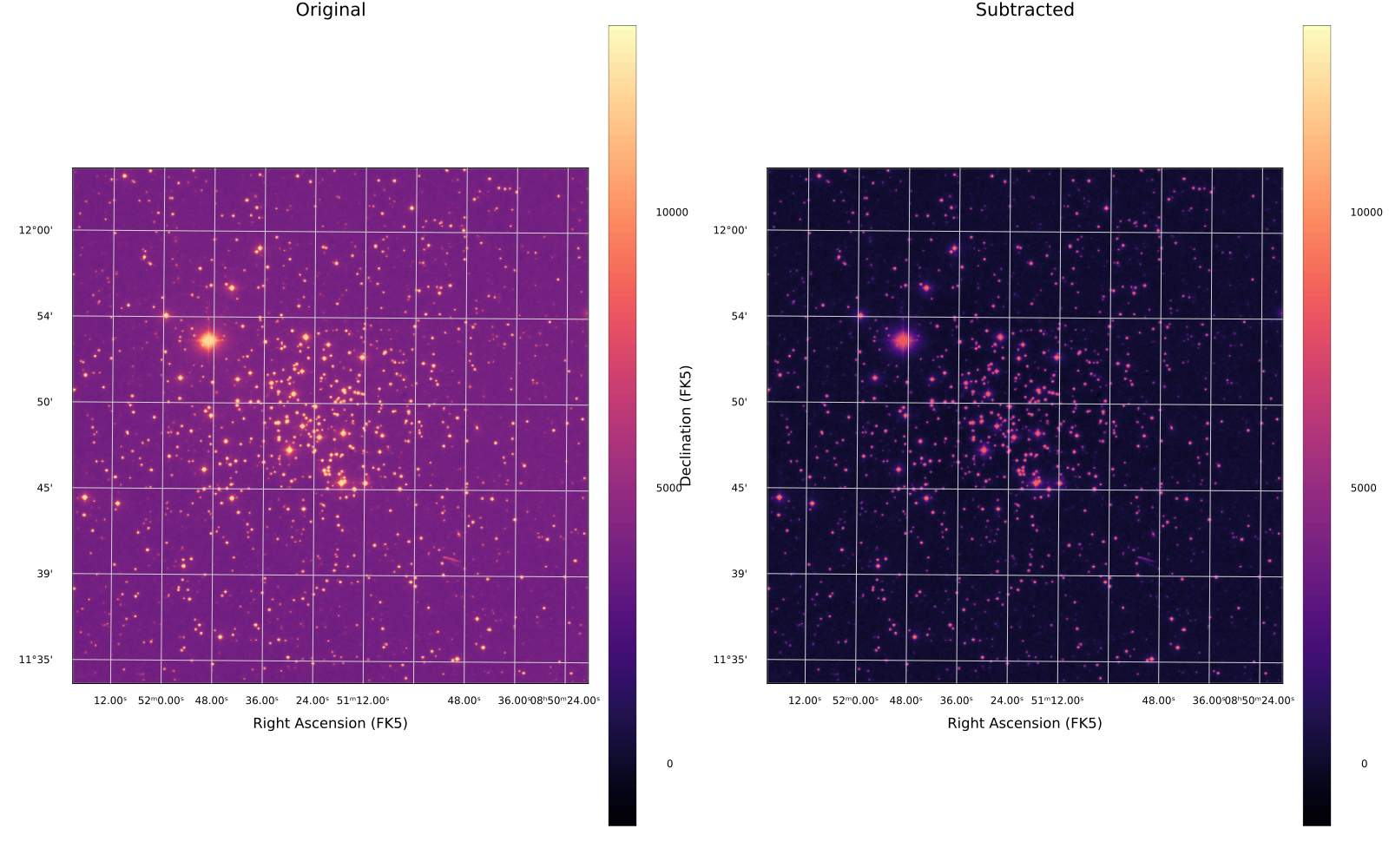
Now we can see our image after subtracting the filtered background and ready for Aperture Photometry!

subt = image .- bkg_f[axes(image)...]
clims = extrema(vcat(vec(image), vec(subt)))
plot(
    implot(image; title = "Original", clims),
    implot(subt; title = "Subtracted", clims);
    size = (1600, 1000),
)

Source Extraction

From the background-subtracted image, we can detect all sources in the image:

# We specify the uncertainty in the pixel data. We'll set it equal to zero.
errs = zeros(axes(subt))
sources = extract_sources(PeakMesh(), subt, errs; sort = true) # sort from brightest to darkest

Table with 3 columns and 57286 rows:
      x     y     value
    ┌────────────────────
 1  │ 226   255   9762.42
 2  │ 681   940   9661.5
 3  │ 924   219   9653.78
 4  │ 678   38    9647.93
 5  │ 85    245   9637.55
 6  │ 1001  44    9633.13
 7  │ 904   503   9627.34
 8  │ 775   819   9625.92
 9  │ 62    610   9617.79
 10 │ 110   133   9616.88
 11 │ 123   592   9614.86
 12 │ 248   1055  9612.46
 13 │ 86    424   9611.86
 14 │ 125   558   9585.93
 15 │ 1021  125   9582.11
 16 │ 637   112   9579.71
 17 │ 2     196   9579.49
 ⋮  │  ⋮     ⋮       ⋮

That's tens of thousands of sources!

We'll define a circular apperture for each source:

aps = CircularAperture.(sources.x, sources.y, 6)[1:1000] # just brightest thousand point sources

1000-element Vector{CircularAperture{Int64}}:
 CircularAperture(226, 255, r=6)
 CircularAperture(681, 940, r=6)
 CircularAperture(924, 219, r=6)
 CircularAperture(678, 38, r=6)
 CircularAperture(85, 245, r=6)
 CircularAperture(1001, 44, r=6)
 CircularAperture(904, 503, r=6)
 CircularAperture(775, 819, r=6)
 CircularAperture(62, 610, r=6)
 CircularAperture(110, 133, r=6)
 ⋮
 CircularAperture(273, 710, r=6)
 CircularAperture(309, 301, r=6)
 CircularAperture(686, 73, r=6)
 CircularAperture(510, 622, r=6)
 CircularAperture(777, 753, r=6)
 CircularAperture(957, 309, r=6)
 CircularAperture(844, 285, r=6)
 CircularAperture(634, 728, r=6)
 CircularAperture(548, 1000, r=6)

We can overplot them on our original image. Photometry.jl uses the same axes convention as AstroImages, with x along the first array axis and y along the second, so the apertures line up with the image as-is:

implot(subt; colorbar = false)
plot!(aps)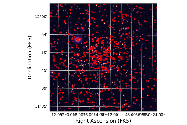

Measuring Photometry

Finally we can extract the source photometry:

table = photometry(aps, subt)

Table with 3 columns and 1000 rows:
      xcenter  ycenter  aperture_sum
    ┌───────────────────────────────
 1  │ 226      255      2.68695e5
 2  │ 681      940      2.35489e5
 3  │ 924      219      3.65716e5
 4  │ 678      38       2.21709e5
 5  │ 85       245      2.4336e5
 6  │ 1001     44       198733.0
 7  │ 904      503      2.25028e5
 8  │ 775      819      3.59414e5
 9  │ 62       610      2.36377e5
 10 │ 110      133      1.60012e5
 11 │ 123      592      3.0983e5
 12 │ 248      1055     2.48006e5
 13 │ 86       424      3.69146e5
 14 │ 125      558      2.87415e5
 15 │ 1021     125      1.83522e5
 16 │ 637      112      2.90848e5
 17 │ 2        196      2.56751e5
 ⋮  │    ⋮        ⋮          ⋮

And plot them:

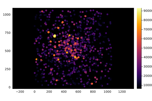
scatter(table.xcenter, table.ycenter;
    aspectratio = 1,
    marker_z = table.aperture_sum,
    markerstrokewidth = 0,
    label = "",
    framestyle = :box,
    background_inside = :black,
    color = :white,
)