Roman

Adapted from STScI Roman Notebooks.

In this example, we show how to use ASDF.jl to load and view some simulated astronomical data created in preparation for the future (Nancy Grace Roman Space Telescope) mission.

Data availability

Simulated data products are currently provided by STScI via AWS S3 buckets. Note: The data product used for this example is a moderately large file (~300 MB).

Load

using ASDF, AWS, AWSS3

fpath = let
    filename = joinpath(mkpath(pkgdir(ASDF, "data")), "roman.asdf")
    path = "roman/nexus/soc_simulations/tutorial_data/r0003201001001001004_0001_wfi01_f106_cal.asdf"
    aws_config = AWS.AWSConfig(; creds = nothing, region = "us-east-1")
    isfile(filename) || s3_get_file(aws_config, "stpubdata", path, filename)
    filename
end

af = load(fpath; extensions = true, validate_checksum = false)

roman.asdf
├─ asdf_library::TaggedMapping
│  ├─ author::String | The ASDF Developers
│  ├─ homepage::String | http://github.com/asdf-format/asdf
│  ├─ name::String | asdf
│  └─ version::String | 4.1.0
├─ history::OrderedDict
│  └─ extensions::Vector{TaggedMapping} | shape = (7,)
└─ roman::TaggedMapping
   ├─ meta::OrderedDict
   │  ├─ asn::OrderedDict
   │  ├─ cal_logs::TaggedSequence | shape = (817,)
   │  ├─ cal_step::TaggedMapping
   │  │  ├─ dq_init::String | COMPLETE
   │  │  ├─ saturation::String | COMPLETE
   │  │  ├─ refpix::String | COMPLETE
   │  │  ├─ linearity::String | COMPLETE
   │  │  ├─ dark::String | COMPLETE
   │  │  ├─ ramp_fit::String | COMPLETE
   │  │  ├─ assign_wcs::String | COMPLETE
  ⋮  (199) more rows

Note

Some ASDF files produced by the Python implementation of ASDF may save a checksum in its header block computed from the original decompressed file. This will cause ASDF.jl to fail because in constrast, it computes the checksum based on the compressed (i.e., "used data"), as per the current specification for ASDF. To handle this potenial failure mode, we pass validate_checksum = false to avoid running the default checksum.

Plot

using CairoMakie

img_sci = let
    img = af["roman"]["data"][]
    @view img[begin:1000, begin:1000]
end

telescope = af["roman"]["meta"]["telescope"]
instr     = af["roman"]["meta"]["instrument"]["name"]
filt      = af["roman"]["meta"]["instrument"]["optical_element"]

fig, ax, hm = heatmap(img_sci;
    axis = (;
        xlabel = "X",
        ylabel = "Y",
        title = "$(telescope) $(instr) -- $(filt)",
    ),
    colorrange = (0.5, 4),
    colorscale = asinh,
    colormap = :cividis,
)

Colorbar(fig[1, 2], hm; label = "Counts")

fig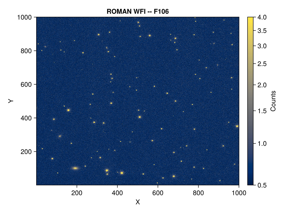

Note

By default, Makie.jl places the origin in the lower left corner and transposes the data, matching the convention used in the Python workshop example. To have the plot orientation match the data orientation instead, modify the above plot command to: heatmap(img_sci'; axis = (; yreversed = true)). See also permutedims for a more general alternative to the adjoint (conjugate transpose) operation: '.