Color laws
The following empirical laws allow us to model the reddening of light as it travels to us. The law you use should depend on the type of data you have and the goal of its use. CCM89 is very common for use in removing extinction from stellar observations, but CAL00, for instance, is suited for galaxies with massive stars. Look through the citations and documentation for each law to get a better idea of what sort of physics it targets.
Usage
Color laws are constructed and then used as a function for passing wavelengths. Wavelengths are assumed to be in units of angstroms.
julia> CCM89(Rv=3.1)(4000)
1.464555702942584
These laws can be applied across higher dimension arrays using the . operator
julia> CCM89(Rv=3.1).([4000, 5000])
2-element Vector{Float64}:
 1.464555702942584
 1.1222468788993019
these laws return magnitudes, which we can apply directly to flux by mulitplication with a base-2.5 logarithmic system (because astronomers are fun):
\[f = f \cdot 10 ^ {-0.4A_v\cdot mag}\]
To make this easier, we provide a convenience redden and deredden functions for applying these color laws to flux measurements.
julia> wave = range(4000, 5000, length=4)
4000.0:333.3333333333333:5000.0

julia> flux = 1e-8 .* wave .+ 1e-2
0.01004:3.3333333333333333e-6:0.01005

julia> redden.(CCM89, wave, flux; Av=0.3)
4-element Vector{Float64}:
 0.00669864601545475
 0.006918253926353551
 0.007154659823737299
 0.007370491272731541

julia> deredden.(CCM89(Rv=3.1), wave, ans; Av=0.3) ≈ flux
true
Advanced Usage
The color laws also have built-in support for uncertainties using Measurements.jl.
julia> using Measurements

julia> CCM89(Rv=3.1).([4000. ± 10.5, 5000. ± 10.2])
2-element Vector{Measurement{Float64}}:
 1.4646 ± 0.0033
 1.1222 ± 0.003
and also support units via Unitful.jl and its subsidiaries. Notice how the output type is now Unitful.Gain.
julia> using Unitful, UnitfulAstro

julia> mags = CCM89(Rv=3.1).([4000u"angstrom", 0.5u"μm"])
2-element Vector{Gain{Unitful.LogInfo{:Magnitude, 10, -2.5}, :?, Float64}}:
 1.464555702942584 mag
 1.1222468788993019 mag
You can even combine the two above to get some really nice workflows exploiting all Julia has to offer! This example shows how you could redden some OIR observational data with uncertainties in the flux density.
julia> using Measurements, Unitful, UnitfulAstro

julia> wave = range(0.3, 1.0, length=5)u"μm"
(0.3:0.175:1.0) μm

julia> err = randn(length(wave))
5-element Vector{Float64}:
 -0.07058313895389791
  0.5314767537831963
 -0.806852326006714
  2.456991333983293
  1.1648740735275196

julia> flux = @.(300 / ustrip(wave)^4 ± err)*u"Jy"
5-element Vector{Quantity{Measurement{Float64}, 𝐌 𝐓^-2, Unitful.FreeUnits{(Jy,), 𝐌 𝐓^-2, nothing}}}:
 37037.037 ± -0.071 Jy
   5893.14 ± 0.53 Jy
   1680.61 ± -0.81 Jy
     647.6 ± 2.5 Jy
     300.0 ± 1.2 Jy

julia> redden.(CCM89, wave, flux; Av=0.3)
5-element Vector{Quantity{Measurement{Float64}, 𝐌 𝐓^-2, Unitful.FreeUnits{(Jy,), 𝐌 𝐓^-2, nothing}}}:
 22410.804 ± 0.043 Jy
   4229.74 ± 0.38 Jy
   1337.12 ± 0.64 Jy
     554.3 ± 2.1 Jy
     268.3 ± 1.0 Jy
Parametric Extinction Laws
These laws are all parametrized by the selective extinction Rv. Mathematically, this is the ratio of the total extinction by the reddening
\[R_V = \frac{A_V}{E(B-V)}\]
and is loosely associated with the size of the dust grains in the interstellar medium.
Index:
Clayton, Cardelli and Mathis (1989)

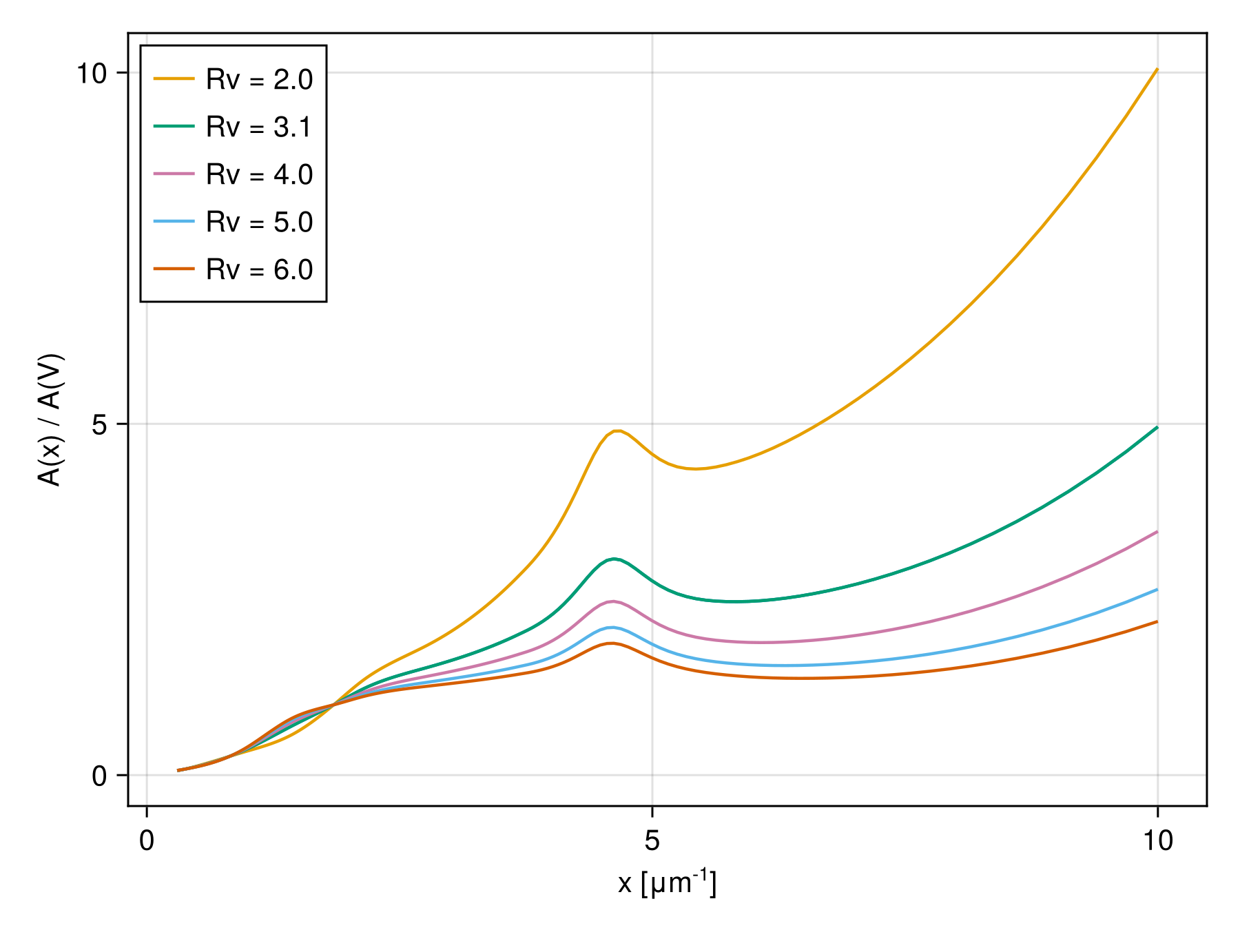
DustExtinction.CCM89 — Type
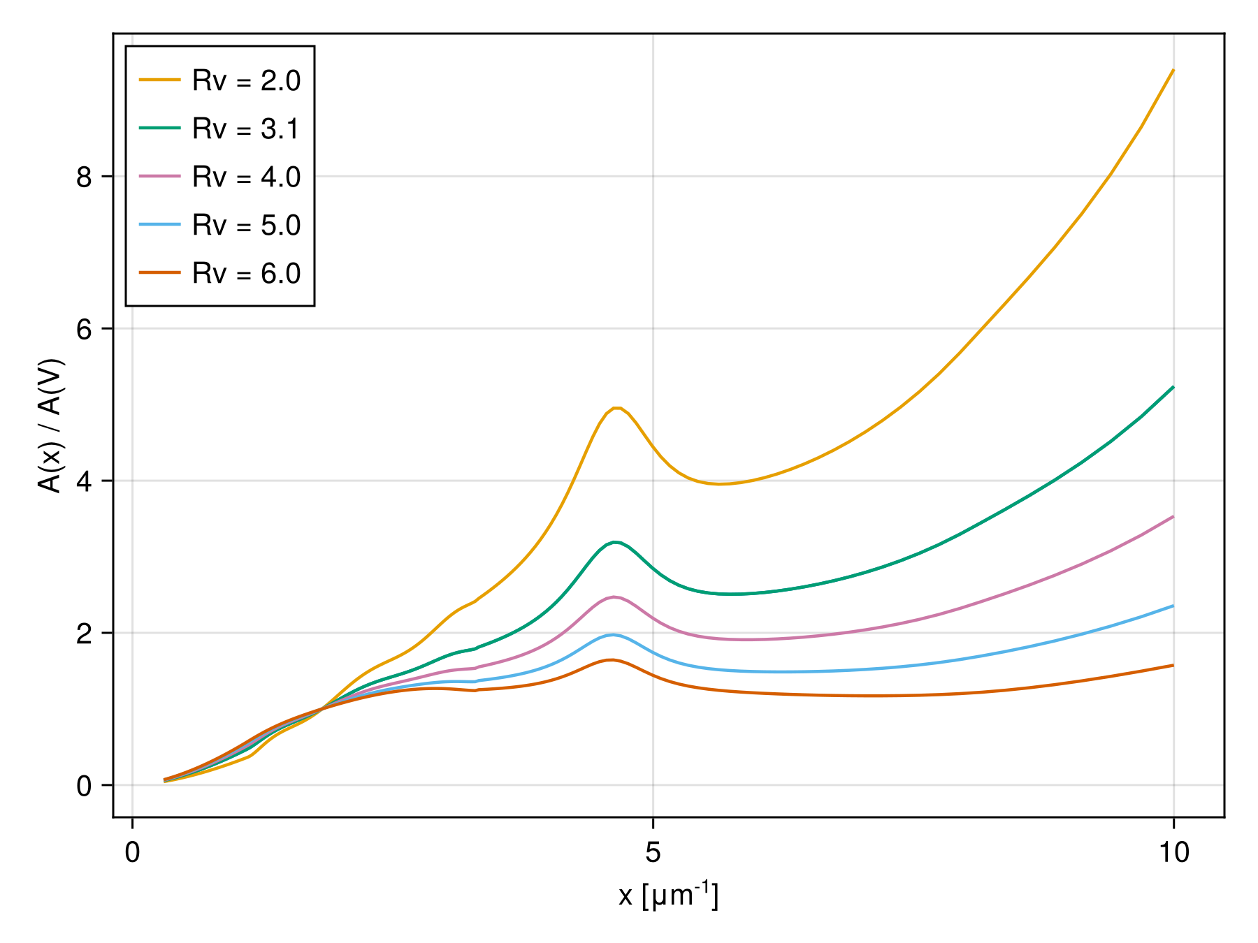
CCM89(;Rv=3.1)Clayton, Cardelli and Mathis (1989) dust law.
Returns A(λ)/A(V) at the given wavelength relative to the extinction at 5494.5 Å. The default support is [1000, 33333]. Outside of that range this will return 0. Rv is the selective extinction and is valid over [2, 6]. A typical value for the Milky Way is 3.1.
References
O'Donnell 1994
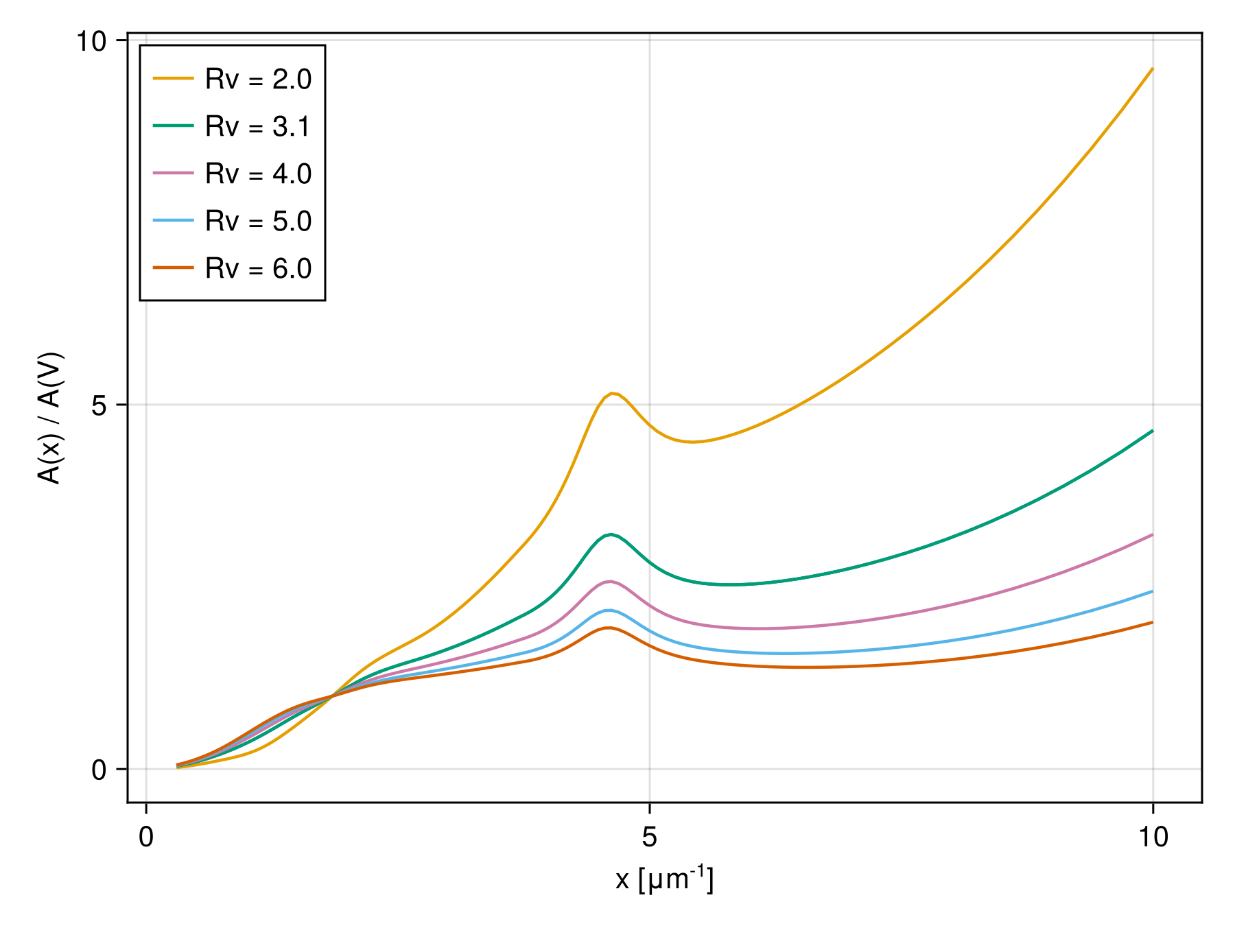
DustExtinction.OD94 — Type
OD94(;Rv=3.1)O'Donnell (1994) dust law.
This is identical to the Clayton, Cardelli and Mathis (1989) dust law, except for different coefficients used in the optical (3030.3 Å to 9090.9 Å).
References
See Also
Calzetti et al. (2000)
DustExtinction.CAL00 — Type
CAL00(;Rv=4.05)Calzetti et al. (2000) Dust Law.
Returns A(λ)/A(V) at the given wavelength. λ is the wavelength in Å and has support over [1200, 22000]. Outside of that range this will return 0.
Calzetti et al. (2000) developed a recipe for dereddening the spectra of galaxies where massive stars dominate the radiation output. They found the best fit value for such galaxies was 4.05±0.80.
References
Valencic, Clayton, & Gordon (2004)
DustExtinction.VCG04 — Type
VCG04(;Rv=3.1)Valencic, Clayton, & Gordon (2004) dust law.
This model applies to the UV spectral region all the way to 912 Å. This model was not derived for the optical or NIR.
References
Gordon, Cartledge, & Clayton (2009)
DustExtinction.GCC09 — Type
GCC09(;Rv=3.1)Gordon, Cartledge, & Clayton (2009) dust law.
This model applies to the UV spectral region all the way to 909.09 Å. This model was not derived for the optical or NIR.
References
Fitzpatrick (1999)
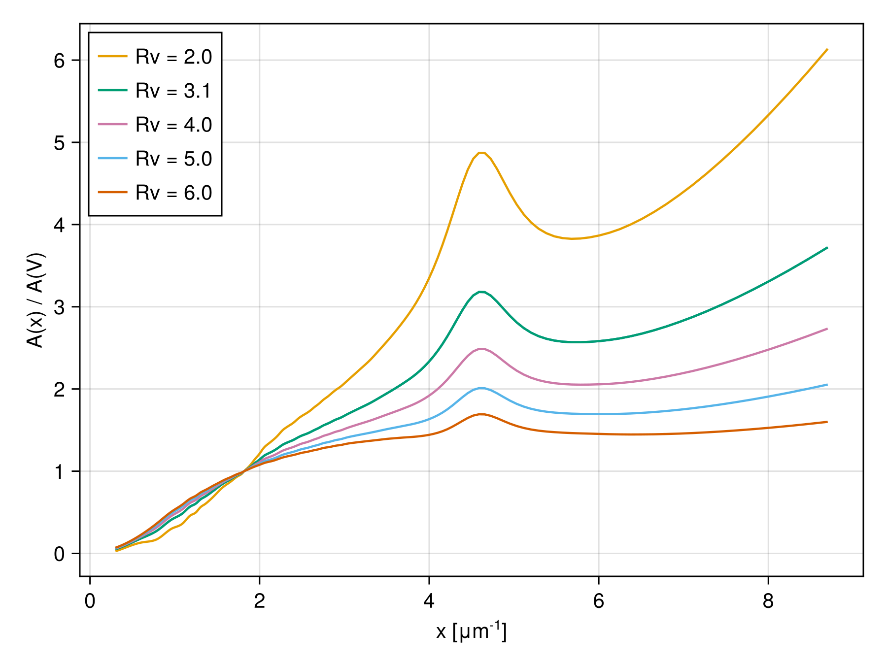
DustExtinction.F99 — Type
F99(;Rv=3.1)Fitzpatrick (1999) dust law.
Returns A(λ)/A(V) at the given wavelength relative to the extinction. This model applies to the UV and optical to NIR spectral range. The default support is [1000, 33333] Å. Outside of that range this will return 0. Rv is the selective extinction and is valid over [2, 6]. A typical value for the Milky Way is 3.1.
References
Fitzpatrick (2004)
DustExtinction.F04 — Type
F04(;Rv=3.1)Fitzpatrick (2004) dust law.
Returns A(λ)/A(V) at the given wavelength relative to the extinction. This model applies to the UV and optical to NIR spectral range. The default support is [1000, 33333] Å. Outside of that range this will return 0. Rv is the selective extinction and is valid over [2, 6]. A typical value for the Milky Way is 3.1.
Equivalent to the F99 model with an updated NIR Rv dependence
See also Fitzpatrick & Massa (2007, ApJ, 663, 320)
References
Fitzpatrick (2019)
DustExtinction.F19 — Type
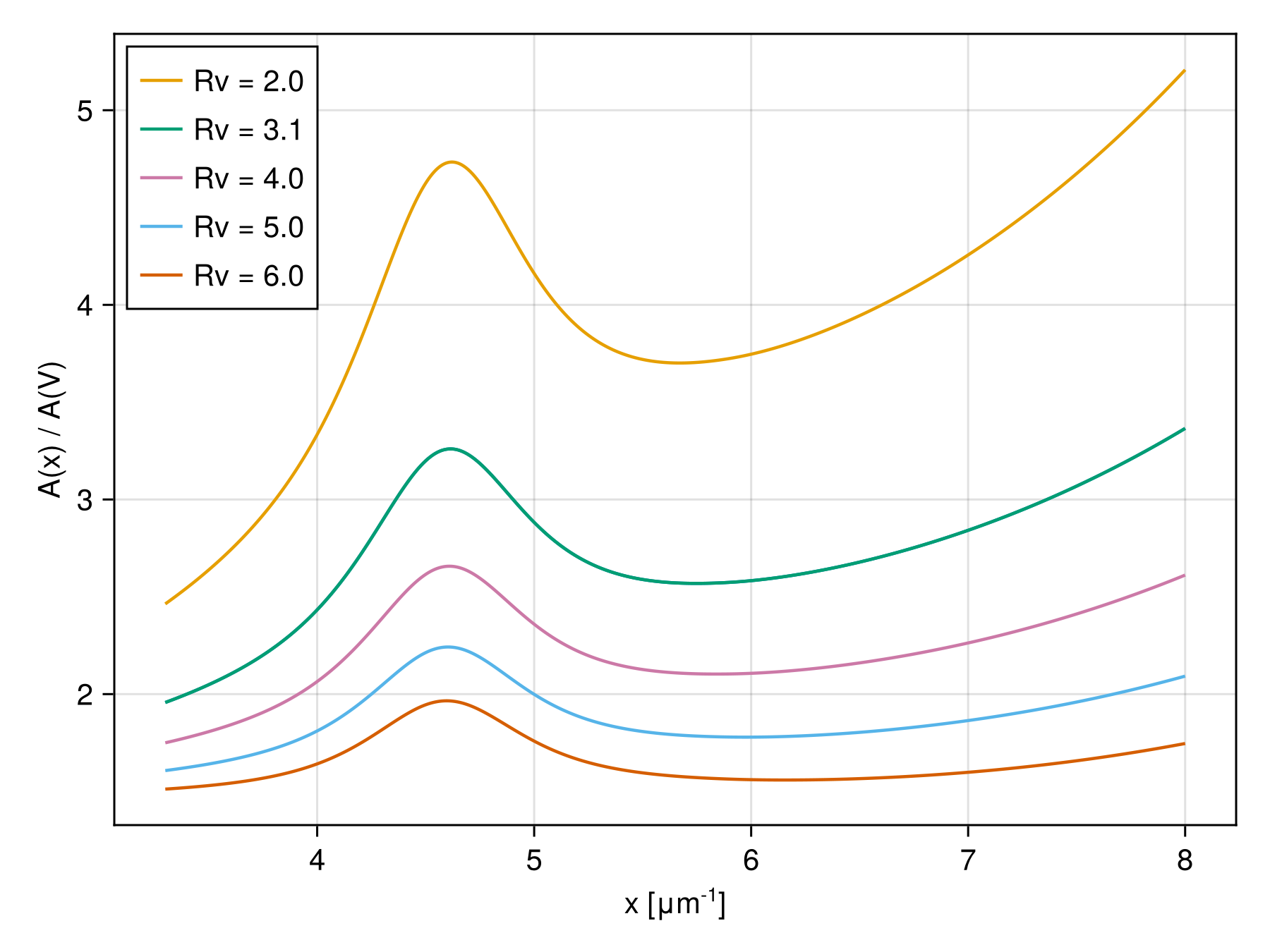
F19(;Rv=3.1)Fitzpatrick (2019) dust law.
Returns A(λ)/A(V) at the given wavelength relative to the extinction. This model applies to the UV and optical to NIR spectral range. The default support is [1149, 33333] Å. Outside of that range this will return 0. Rv is the selective extinction and is valid over [2, 6]. A typical value for the Milky Way is 3.1.
Fitzpatrick, Massa, Gordon et al. (2019, ApJ, 886, 108) model. Based on a sample of stars observed spectroscopically in the optical with HST/STIS.
References
Maiz Apellaniz et al. (2014)
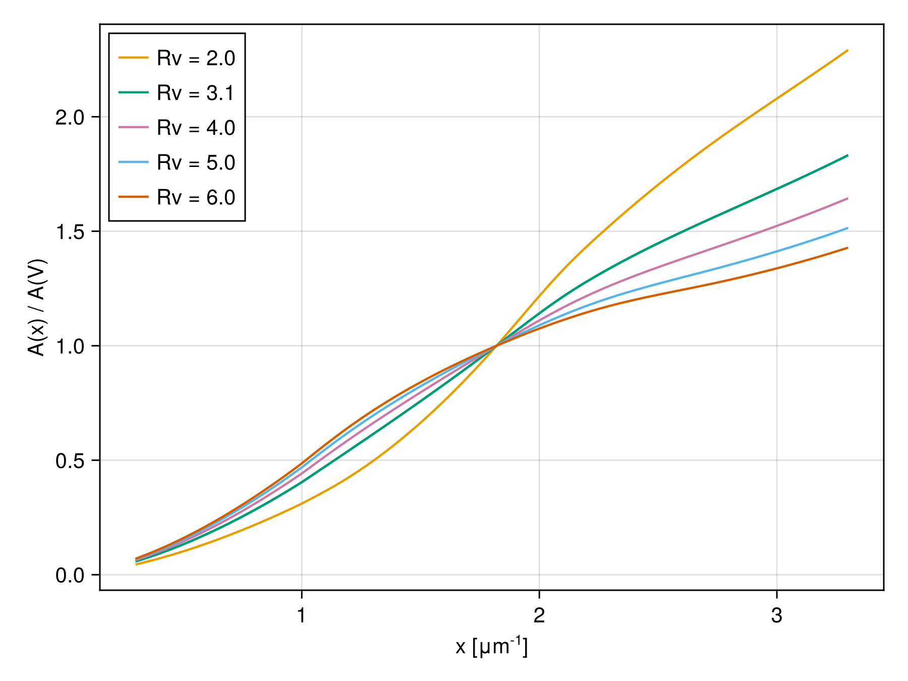
DustExtinction.M14 — Type
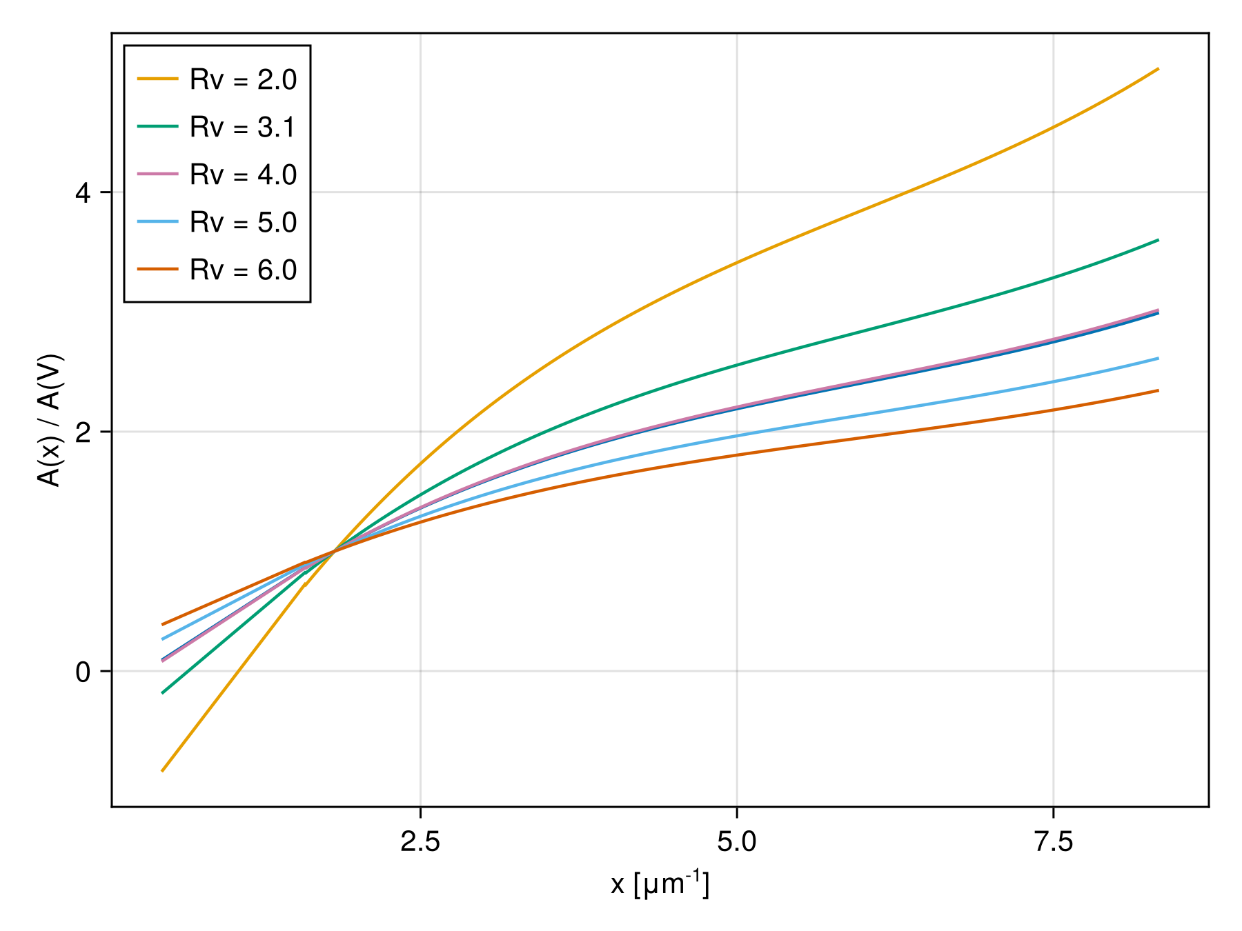
M14(;Rv=3.1)Maiz Apellaniz et al (2014) Milky Way & LMC R(V) dependent model.
Returns A(λ)/A(V) at the given wavelength relative to the extinction. The published UV extinction curve is identical to Clayton, Cardelli, and Mathis (1989, CCM). Forcing the optical section to match smoothly with CCM introduces a non-physical feature at high values of R5495 around 3.9 inverse microns; see section 5 in Maiz Apellaniz et al. (2014) for more discussion. For that reason, we provide the M14 model only through 3.3 inverse microns, the limit of the optical in CCM. Outside of that range this will return 0. Rv is the selective extinction and is valid over [2, 6]. A typical value for the Milky Way is 3.1. R5495 = A(5485)/E(4405-5495) Spectral equivalent to photometric R(V).
References
Fittable Extinction Laws
Fitzpatrick & Massa (1990)
DustExtinction.FM90 — Type
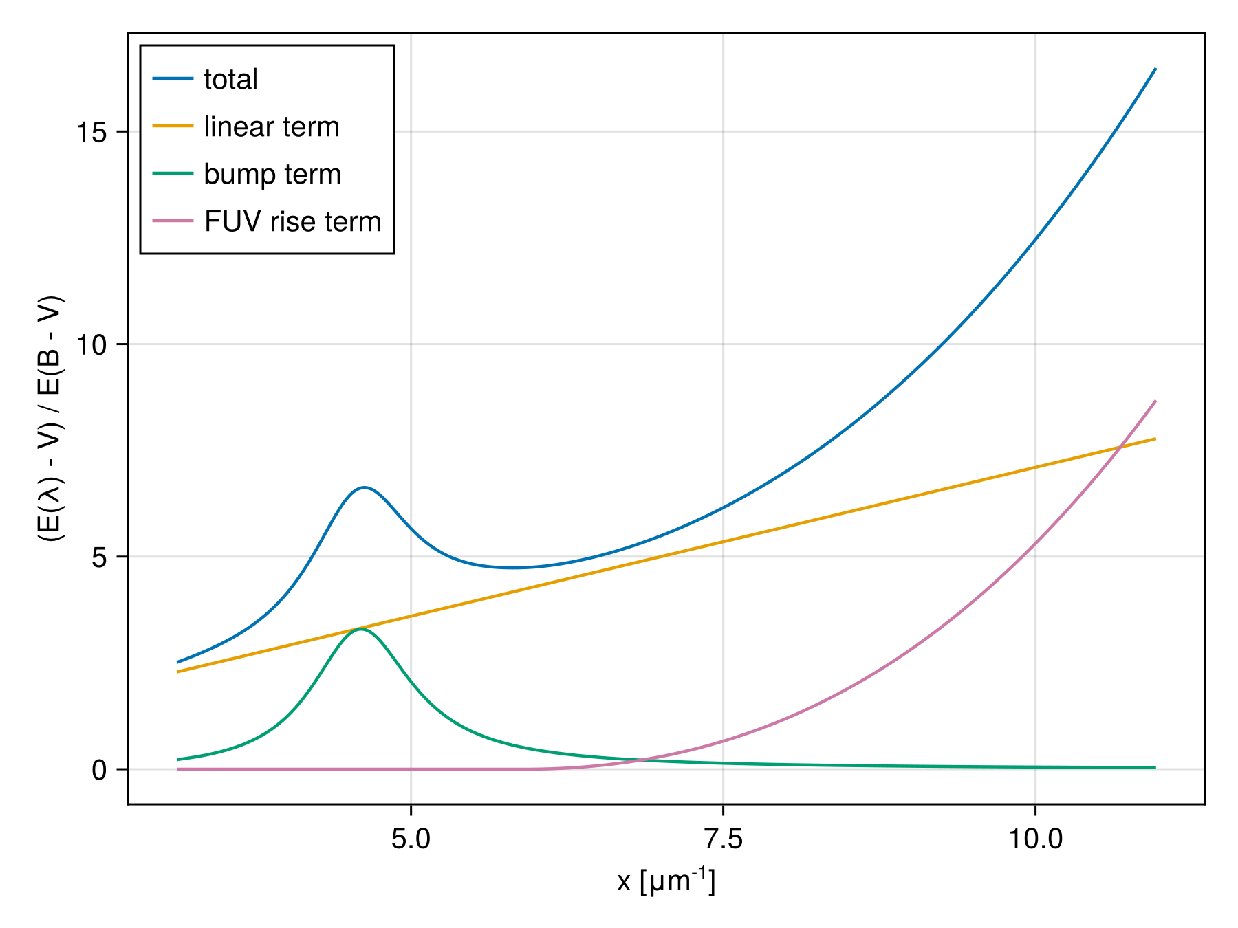
FM90(;c1=0.10, c2=0.70, c3=3.23, c4=0.41, x0=4.60, gamma=0.9)
FM90(coeffs, x0=4.60, gamma=0.9)
Fitzpatrick & Massa (1990) generative model for ultraviolet dust extinction. The default values are the published values for the Milky Way average.
Parameters
c1- y-intercept of linear termc2- slope of liner termc3- amplitude of 2175 Å bumpc4- amplitude of FUV risex0- centroid of 2175 Å bumpgamma- width of 2175 Å bump
If λ is a Unitful.Quantity it will be automatically converted to Å and the returned value will be UnitfulAstro.mag.
Examples
julia> model = FM90(c1=0.2, c2=0.7, c3=3.23, c4=0.41, x0=4.6, gamma=0.99);

julia> model(1500)
5.2521258452800135

julia> FM90()(1500)
5.152125845280013

julia> FM90(c1=0.2, c2=0.7, c3=3.23, c4=0.41, x0=4.6, gamma=0.99).([1000, 1200, 1800])
3-element Vector{Float64}:
 12.562237969522851
  7.769215017329513
  4.890128210972148
Extended Help
The model has form $c_1 + c_2x + c_3D(x; γ, x_0) + c_4 F(x)$ where $x$ is the wavenumber in inverse microns, $D(x)$ is a Drude profile (modified Lorentzian) used to model the 2175 Å bump with the scale-free parameters $x_0$ (central wavenumber) and $γ$ (damping coefficient), and $F(x)$, a piecewise function for the far-UV. Note that the coefficients will change the overall normalization, possibly changing the expected behavior of reddening via the parameter $A_V$.
References
Pei (1992)
DustExtinction.P92 — Type
P92(; BKG_amp=218.57,  BKG_lambda=0.047, BKG_b=90.0,   BKG_n=2.0,
      FUV_amp=18.54,   FUV_lambda=0.08,  FUV_b=4.0,    FUV_n=6.5,
      NUV_amp=0.0596,  NUV_lambda=0.22,  NUV_b=-1.95,  NUV_n=2.0,
      SIL1_amp=0.0026, SIL1_lambda=9.7,  SIL1_b=-1.95, SIL1_n=2.0,
      SIL2_amp=0.0026, SIL2_lambda=18.0, SIL2_b=-1.8,  SIL2_n=2.0,
      FIR_amp=0.0159,  FIR_lambda=25.0,  FIR_b=0.0,    FIR_n=2.0)
Pei (1992) generative extinction model applicable from the extreme UV to far-IR.
Parameters
Background Terms
BKG_amp- amplitudeBKG_lambda- central wavelengthBKG_b- b coefficientBKG_n- n coefficient
Far-Ultraviolet Terms
FUV_amp- amplitudeFUV_lambda- central wavelengthFUV_b- b coefficentFUV_n- n coefficient
Near-Ultraviolet (2175 Å) Terms
NUV_amp- amplitudeNUV_lambda- central wavelengthNUV_b- b coefficentNUV_n- n coefficient
1st Silicate Feature (~10 micron) Terms
SIL1_amp- amplitudeSIL1_lambda- central wavelengthSIL1_b- b coefficentSIL1_n- n coefficient
2nd Silicate Feature (~18 micron) Terms
SIL2_amp- amplitudeSIL2_lambda- central wavelengthSIL2_b- b coefficientSIL2_n- n coefficient
Far-Infrared Terms
FIR_amp- amplitudeFIR_lambda- central wavelengthFIR_b- b coefficentFIR_n- n coefficient
If λ is a Unitful.Quantity it will be automatically converted to Å and the returned value will be UnitfulAstro.mag.
Examples
julia> model = P92();

julia> model(1500)
2.561019978746464

julia> P92(FUV_b = 2.0).([1000, 2000, 3000])
3-element Vector{Float64}:
 5.17952309549434
 2.7581232249728607
 1.8081781540687367
Default Parameter Values
| Term | lambda (μm) | A | b | n |
|---|---|---|---|---|
| BKG | 0.047 | 218.57142857142858 | 90.0 | 2.0 |
| FUV | 0.08 | 18.545454545454547 | 4.0 | 6.5 |
| NUV | 0.22 | 0.05961038961038961 | -1.95 | 2.0 |
| SIL1 | 9.7 | 0.0026493506493506496 | -1.95 | 2.0 |
| SIL2 | 18.0 | 0.0026493506493506496 | -1.8 | 2.0 |
| FIR | 25.0 | 0.015896103896103898 | 0.0 | 2.0 |
References
Mixture Extinction Laws
Gordon et al. (2003)
DustExtinction.G03_SMCBar — Type
G03_SMCBar(;Rv=2.74) <Internal function>Gordon et al. (2003) SMCBar Average Extinction Curve.
The observed A(lambda)/A(V) values at 2.198 and 1.25 microns were changed to provide smooth interpolation as noted in Gordon et al. (2016, ApJ, 826, 104)
Reference
DustExtinction.G03_LMCAve — Type
G03_LMCAve(;Rv=3.41) <Internal function>Gordon et al. (2003) LMCAve Average Extinction Curve.
Reference
Gordon et al. (2016)
DustExtinction.G16 — Type
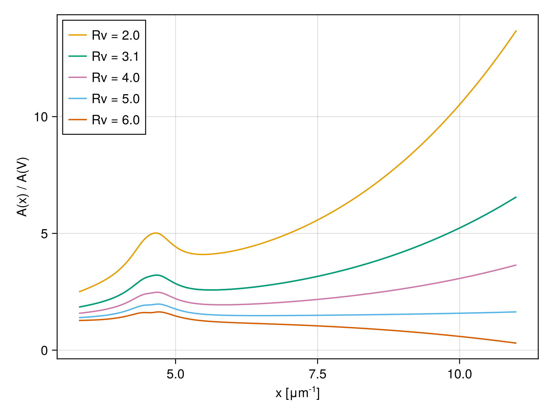
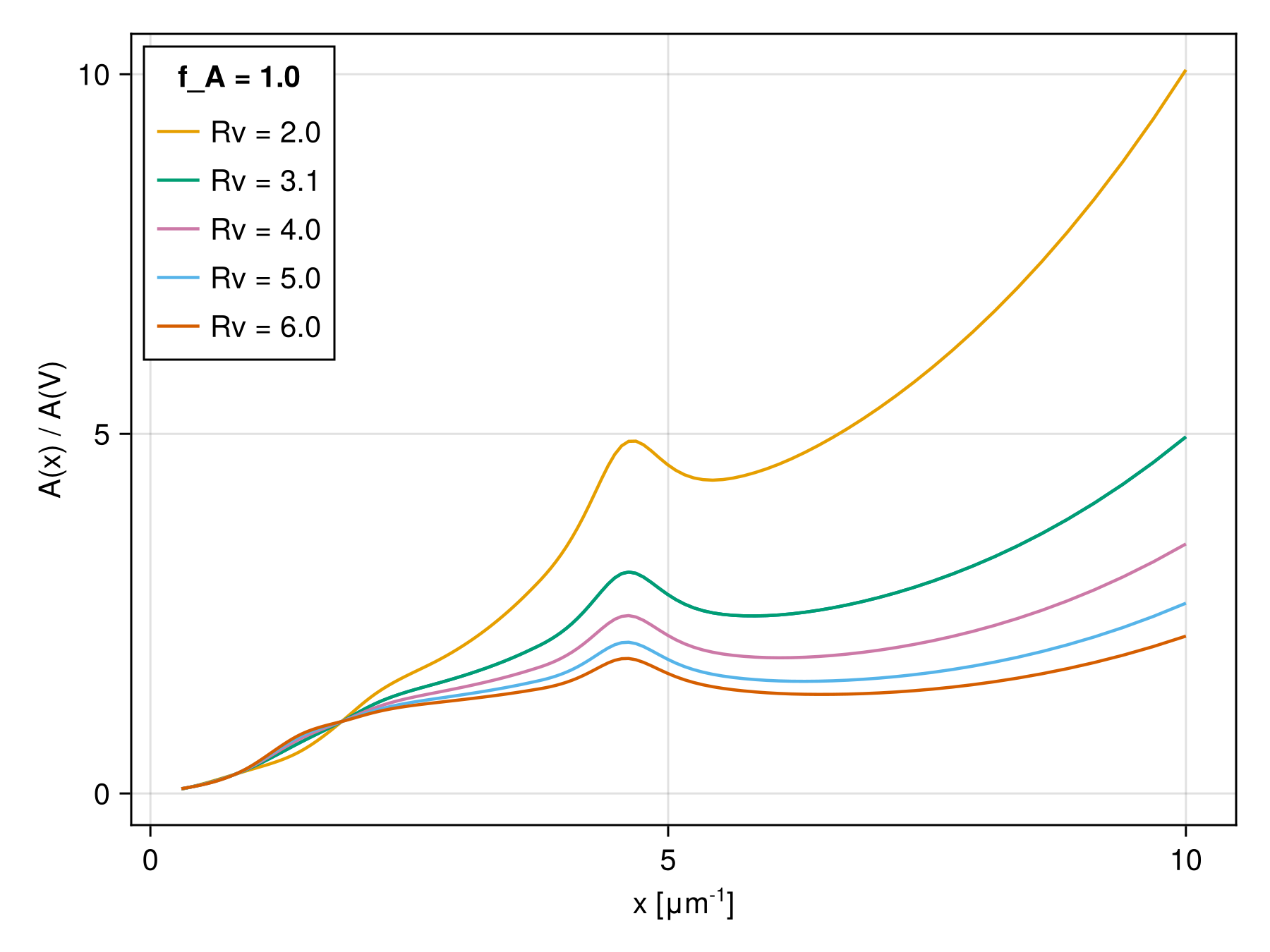
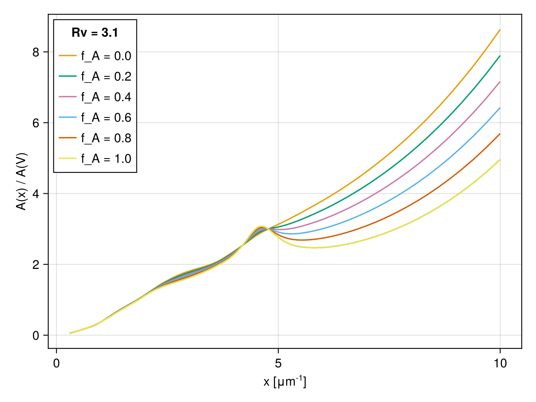
G16(;Rv=3.1, f_A=1.0)Gordon et al. (2016) Milky Way, LMC, & SMC R(V) and f_A dependent model
Returns A(λ)/A(V) at the given wavelength relative to the extinction. This is mixture model between the F99 R(V) dependent model (component A) and the G03_SMCBar model (component B). The default support is [1000, 33333] Å. Outside of that range this will return 0. Rv is the selective extinction and is valid over [2, 6]. A typical value for the Milky Way is 3.1.
References
API/Reference
DustExtinction.redden — Function
redden(::ExtinctionLaw, wave, flux; Av=1)
redden(::Type{ExtinctionLaw}, wave, flux; Av=1, law_kwargs...)
Redden the given flux using the given extinction law at the given wavelength.
If wave is <:Real then it is expected to be in angstrom and if it is <:Unitful.Quantity it will be automatically converted. Av is the total extinction value. The extinction law can be a constructed struct or a Type. If it is a Type, law_kwargs will be passed to the constructor.
Examples
julia> wave = 3000; flux = 1000;

julia> redden(CCM89, wave, flux; Rv=3.1)
187.38607779757183

julia> redden(CCM89(Rv=3.1), wave, flux; Av=2)
35.11354215235764
See Also
DustExtinction.redden! — Function
redden!(::ExtinctionLaw, wave, flux; Av=1)
redden!(::Type{ExtinctionLaw}, wave, flux; Av=1, law_kwargs...)
In-place version of redden. Modifies flux.
DustExtinction.deredden — Function
deredden(::ExtinctionLaw, wave, flux; Av=1)
deredden(::Type{ExtinctionLaw}, wave, flux; Av=1, law_kwargs...)
Deredden the given flux using the given extinction law at the given wavelength.
If wave is <:Real then it is expected to be in angstrom and if it is <:Unitful.Quantity it will be automatically converted. Av is the total extinction value. The extinction law can be a constructed struct or a Type. If it is a Type, law_kwargs will be passed to the constructor.
Examples
julia> wave = 3000; flux = 187.386;

julia> deredden(CCM89, wave, flux; Rv=3.1)
999.9995848273642

julia> deredden(CCM89(Rv=3.1), wave, flux; Av=2)
5336.573541539394
See Also
DustExtinction.deredden! — Function
deredden!(::ExtinctionLaw, wave, flux; Av=1)
deredden!(::Type{ExtinctionLaw}, wave, flux; Av=1, law_kwargs...)
In-place version of deredden. Modifies flux.
DustExtinction.ExtinctionLaw — Type
abstract type DustExtinction.ExtinctionLawThe abstract supertype for dust extinction laws. See the extended help (??DustExtinction.ExtinctionLaw from the REPL) for more information about the interface.
Extended Help
Interface
Here's how to make a new extinction law, called MyLaw
- Create your struct. We strongly recommend using keyword arguments if your model is parameterized, which allows convenient usage with
reddenandderedden.struct MyLaw <: DustExtinction.ExtinctionLaw end - (Optional) Define the limits. This will default to
(0, Inf). Currently, this is used within theDustExtinction.checkboundsfunction and in the future will be used for plotting recipes.DustExtinction.bounds(::Type{<:MyLaw}) = (min, max) - Define the law. You only need to provide one function which takes wavelength as angstrom. If your law is naturally written for inverse-micron, there is a helper function
aa_to_invum.(::MyLaw)(wavelength::Real) - (Optional) enable
Unitful.jlsupport by adding this function. If you are building a new law withinDustExtinction.jlyou can add your law to the code-gen list insideDustExtinction.jl/src/DustExtinction.jl.(l::MyLaw)(wavelength::Unitful.Quantity) = l(ustrip(u"angstrom", wavelength)) * u"mag"
DustExtinction.bounds — Function
DustExtinction.bounds(::ExtinctionLaw)::Tuple
DustExtinction.bounds(::Type{<:ExtinctionLaw})::Tuple
Get the natural wavelengths bounds for the extinction law, in angstrom
DustExtinction.checkbounds — Function
DustExtinction.checkbounds(::ExtinctionLaw, wavelength)::Bool
DustExtinction.checkbounds(::Type{<:ExtinctionLaw, wavelength}::Bool
Helper function that uses DustExtinction.bounds to return whether the given wavelength is in the support for the law.