Dimensions and World Coordinates
AstroImages are based on Dimensional Data. Each axis is assigned a dimension name and the indices are tracked.
World Coordinates
FITS files with world coordinate system (WCS) headers contain all the information necessary to map a pixel location into celestial coordinates & back.
Let's see how this works with a 2D image with RA & DEC coordinates.
using AstroImages
using Plots

# Download a Hubble image of the Eagle nebula
download(
    "https://ds9.si.edu/download/data/656nmos.fits",
    "eagle-656nmos.fits"
);
eagle = load("eagle-656nmos.fits")
This image contains world coordinate system headers. AstroImages.jl uses WCS.jl (and wcslib under the hood) to parse these headers. We can generate a WCSTransform object to inspect:
wcs(eagle, 1) # specify which coordinate systemWCSTransform(naxis=2,cdelt=[1.0, 1.0],crval=[274.71149247724, -13.816384007184],crpix=[386.5, 396.0])Note that we specify with an index which coordinate system we'd like to use. Most images just contain one, but some contain multiple systems.
We can lookup a coordinate from the image:
world = pix_to_world(eagle, [1, 1]) # Bottom left corner2-element Vector{Float64}:
274.712299241082
-13.801135972688115Or convert back from world coordinates to pixel coordinates: We can lookup a coordinate from the image:
world_to_pix(eagle, world) # Bottom left corner2-element Vector{Float64}:
1.000000000336172
0.9999999992196535These pixel coordinates do not necessarily have to lie within the bounds of the original image, and in general lie at a fractional pixel position.
If an image contains WCS headers, we can visualize them using implot:
implot(eagle)
We can adjust the color of the grid:
implot(eagle, gridcolor=:cyan)
If these aren't desired, we can turn off the grid or the WCS tick marks:
plot(
  implot(eagle, grid=false),
  implot(eagle, wcsticks=false),
  size=(900,300),
  bottommargin=10Plots.mm
)
Since AstroImages are based on DimensionalData's AbstractDimArray, the mapping between pixel coordinates and world coordinates are preserved when slicing an AstroImage:
slice1 = eagle[1:800,1:800]
slice2 = eagle[800:1600,1:800]
plot(
  implot(slice1),
  implot(slice2),
  size=(900,300),
  bottommargin=10Plots.mm
)
World coordinate queries from that slice are aware of their position in the parent image:
@show pix_to_world(slice1, [1,1])2-element Vector{Float64}:
274.712299241082
-13.801135972688115@show pix_to_world(slice2, [1,1])2-element Vector{Float64}:
274.7277517847315
-13.817350009028138Note that you can query the dimensions of an image using the dims function from DimensionalData:
dims(slice2)(↓ X Sampled{Int64} 800:1600 ForwardOrdered Regular Points,
→ Y Sampled{Int64} 1:800 ForwardOrdered Regular Points)Named Dimensions
Each dimension of an AstroImage is named. The automatic dimension names are X, Y, Z, Dim{4}, Dim{5}, and so on; however you can pass in other names or orders to the load function and/or AstroImage contructor:
julia> img = load("eagle-656nmos.fits", 1, (Y,Z))
1600×1600 AstroImage{Float32,2} with dimensions:
  Y Sampled 1:1600 ForwardOrdered Regular Points,
  Z Sampled 1:1600 ForwardOrdered Regular Points
Other useful dimension names are Spec for spectral axes, Pol for polarization data, and Ti for time axes. These are tracked the same way as the automatic dimension names and interact smoothly with any WCS headers. You can give a dimension an arbitrary name using Dim{Symbol}, e.g., Dim{:Velocity}.
You can access AstroImages using dimension names:
eagle[X=100]╭────────────────────────────────────╮
│ 1600-element AstroImage{Float32,1} │
├────────────────────────────────────┴─────────────────────────────────── dims ┐
↓ Y Sampled{Int64} 1:1600 ForwardOrdered Regular Points
└──────────────────────────────────────────────────────────────────────────────┘
1 0.0
2 0.0
3 0.0
4 0.0
5 0.0
6 0.0
⋮
1596 0.0
1597 0.0
1598 0.0
1599 0.0
1600 0.0When indexing into a slice out of a larger parent image or cube, this named access refers to the parent dimensions:
slice1 = eagle[600:800,600:800]
slice1[X=At(700),Y=At(700)] == eagle[X=At(700),Y=At(700)] == eagle[700,700]trueCubes
Let's see how this works with a 3D cube.
using AstroImages

HIcube = load(download("https://www.astropy.org/astropy-data/tutorials/FITS-cubes/reduced_TAN_C14.fits"))
╭───────────────────────────────────╮
│ 150×150×450 AstroImage{Float32,3} │
├───────────────────────────────────┴──────────────────────────────────── dims ┐
↓ X Sampled{Int64} Base.OneTo(150) ForwardOrdered Regular Points,
→ Y Sampled{Int64} Base.OneTo(150) ForwardOrdered Regular Points,
↗ Z Sampled{Int64} Base.OneTo(450) ForwardOrdered Regular Points
└──────────────────────────────────────────────────────────────────────────────┘
[:, :, 1]
↓ → 1 2 3 4 5 6 … 144 145 146 147 148 149 150
1 NaN NaN NaN NaN NaN NaN NaN NaN NaN NaN NaN NaN NaN
2 NaN NaN NaN NaN NaN NaN NaN NaN NaN NaN NaN NaN NaN
3 NaN NaN NaN NaN NaN NaN NaN NaN NaN NaN NaN NaN NaN
4 NaN NaN NaN NaN NaN NaN NaN NaN NaN NaN NaN NaN NaN
⋮ ⋮ ⋱ ⋮ ⋮
147 NaN NaN NaN NaN NaN NaN NaN NaN NaN NaN NaN NaN NaN
148 NaN NaN NaN NaN NaN NaN NaN NaN NaN NaN NaN NaN NaN
149 NaN NaN NaN NaN NaN NaN NaN NaN NaN NaN NaN NaN NaN
150 NaN NaN NaN NaN NaN NaN … NaN NaN NaN NaN NaN NaN NaNNotice how the cube is not displayed automatically. We have to pick a specific slice:
HIcube[Z=228]
Using implot, the world coordinates are displayed automatically:
implot(HIcube[Z=228], cmap=:turbo)
The plot automatically reflects the world coordinates embeded in the file. It displays the x axis in galactic longitude, the y-axis in galactic latitude, and even shows the curved projection from pixel coordinates to galactic coordinates. The title is automatically set to the world coordinate along the Z axis in units of velocity. It also picks up the unit of the data (Kelvins) to display on the colorbar.
If we pick another slice, the title updates accordingly:
implot(HIcube[Z=308], cmap=:turbo)
This works for other slices through the cube as well:
implot(HIcube[Y=45], cmap=:turbo, aspectratio=0.3)
Custom Dimensions
julia> img = load("img.fits",1,(Y=1:1600,Z=1:1600))
1600×1600 AstroImage{Float32,2} with dimensions:
  Y Sampled 1:1600 ForwardOrdered Regular Points,
  Z Sampled 1:1600 ForwardOrdered Regular Points
Other useful dimension names are Spec for spectral axes, Pol for polarization data, and Ti for time axes. These are tracked the same was as the automatic dimension names and interact smoothly with any WCS headers.
Often times we have images or cubes that we want to index with physical coordinates where setting up a full WCS transform is overkill. In these cases, it's easier to leverage custom dimensions.
For example, one may wish to
julia> img = load("img.fits",1,(X=801:2400,Y=1:2:3200))
1600×1600 AstroImage{Float32,2} with dimensions:
  X Sampled 801:2400 ForwardOrdered Regular Points,
  Y Sampled 1:2:3199 ForwardOrdered Regular Points
...
Unlike OffsetArrays, the usual indexing remains so img[1,1] is still the bottom left of the image; however, data can be looked up according to the offset dimensions using specifiers:
julia> img[X=Near(2000),Y=1..100]
50-element AstroImage{Float32,1} with dimensions:
  Y Sampled 1:2:99 ForwardOrdered Regular Points
and reference dimensions:
  X Sampled 2000:2000 ForwardOrdered Regular Points
  0.0
You can adjust the center of an image's dimensions using recenter:
eagle_cen = recenter(eagle, 801, 801);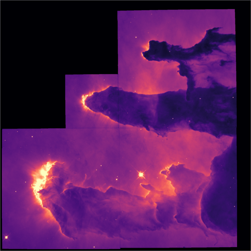
Unlike an OffsetArray, eagle_cen[1,1] still refers to the bottom left of the image. This also has no effect on broadcasting; eagle_cen .+ ones(1600,1600) is perfectly valid. However, we see the new centered dimensions when we go to plot the image:
implot(eagle_cen, wcsticks=false)
And we can query positions using the offset dimensions:
implot(eagle_cen[X=-300..300, Y=-300..300], wcsticks=false)